The theory of evolution is based on the principle that organisms whose heritable traits confer greater fitness have a greater tendency to survive and reproduce. This notion is often presented and understood qualitatively, but I believe there is value in also studying it mathematically. In this article, I develop mathematical models for phenotypic and genotypic changes over time in large populations. In addition to demonstrating the validity of the principles of evolutionary theory, mathematical modelling can elucidate aspects of evolution and population dynamics not observable experimentally.
Model of a binary system
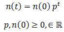
The simplest possible case is where there are only two phenotypes organisms can have, a binary system. Suppose the organisms in a species have a single variable heritable trait. An organism can have either the A or B phenotype for this trait, each of which confer a different degree of fitness (p) to the organism. Fitness denotes the probability of it surviving and/or proliferating per unit of time. The death of organisms is probabilistic. Thus, the development of a model of the population can greatly simplified by assuming an infinite population size. By the Law of Large Numbers, the outcome must be the probabilistically expected result. This assumption also means that the absolute number of a given organism class need not be considered; only the relative ratio is important. The number of organism with a given phenotype (n) can be expressed as a function of time (t) as:
This equation predicts that number of organisms with of a particular fitness would approach 0 when p<1 or infinity when p>1, which does not sound reasonable. Real populations tend to be stable, growing until reaching some maximum carrying capacity. However, as I stated above only the ratio between the amounts of each class of organism are meaningful since we are assuming the population is infinite. Nevertheless, we could include an addition factor to the calculation of n(t) to maintain the population ‘s total size (N) around some carrying capacity (K):
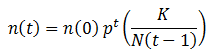
However, we are only concerned with the relative proportion of each phenotype since we are assuming that the population is large. Thus, this carrying capacity term can be neglected.
We can follow the relative amount of each phenotype simply by computing the ratio of the number of organisms with that phenotype to the total size of the population. For instance, the relative amount (A) of phenotype A is given by:
We can follow the relative amount of each phenotype simply by computing the ratio of the number of organisms with that phenotype to the total size of the population. For instance, the relative amount (A) of phenotype A is given by:
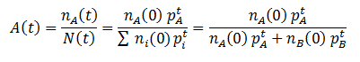
Note that nA(0) and nB(0) refer to the relative initial amounts of the phenotypes, rather than the actual number of organism with each.
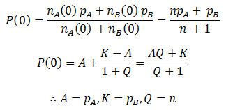
Similarly, we can monitor the average fitness of the population as a function of time by taking a weighted average of the fitness levels present in the population:
Similarly, we can monitor the average fitness of the population as a function of time by taking a weighted average of the fitness levels present in the population:

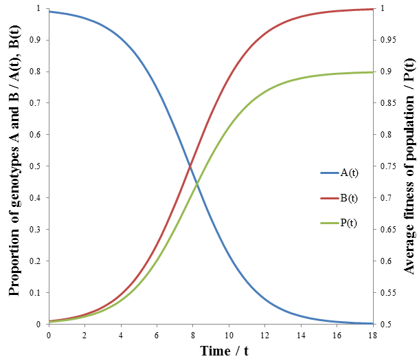
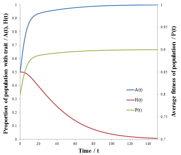
The behavior of these equations can be more readily understood with an example. Suppose we have a population with an equal ratio of organisms with phenotypes A and B which confer fitness values of 0.5 and 0.9 respectively. This gives:
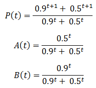
A plot of these equations follows below:
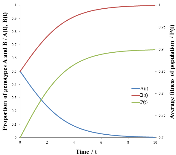
The less fit organisms (phenotype A, p=0.5) die off selectively enriching the remaining population in fit organisms (phenotype B, p=0.9), causing the fitness to converge to 0.9. This is the basis of how natural selection leads to greater fitness of a species. The rate of increase of P(t) is greatest at the beginning (t=0). However, this is not always the case for this model. Consider a population with a 100:1 ratio of organisms with phenotypes A and B, having the same fitness values as before. Then we have:
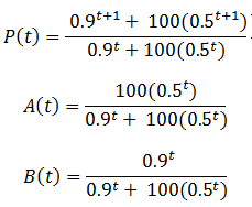
These equations are plotted in the following figure:
The growth in fitness, P(t), is now sigmoidal. The rate at which unfit organisms (phenotype A, p=0.5) die is greatest at the beginning though, since the number dying is proportional to the number in the group. However, because they so greatly outnumber the fit organisms (phenotype B, p=0.9) by a 100:1 ratio their initial deaths have only a small effect on the average fitness. Thus, the rate of increase of average fitness is maximum when the ratio of fit to unfit organisms is no longer small. The rate falls past this point as the population becomes depleted of unfit organisms. Visually, the rate of average fitness increase appears to be maximum when there are equal proportions of organisms A and B. Note that the inflexion point of P(t) occurs at the same time as when A(t) and B(t) intersect. I will show that this is indeed the case mathematically by finding the second derivative of P(t) and solving for its roots to give the inflexion point.
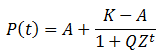
In its present form however, differentiation of P(t) gives a complicated function which is difficult to analyze. The sigmoidal shape is consistent with a logistic curve, whose form is simpler and more feasible to differentiate. Thus I attempted to find an equivalent form of P(t) in terms of the generalized logistic equation:
In its present form however, differentiation of P(t) gives a complicated function which is difficult to analyze. The sigmoidal shape is consistent with a logistic curve, whose form is simpler and more feasible to differentiate. Thus I attempted to find an equivalent form of P(t) in terms of the generalized logistic equation:
Most of the parameters in this equation for P(t) can be found immediately by comparing the expression of the previous equation for P(t) at t=0 to the generalized logistic equation at t=0. For simplicity, let n=nA(0)/nB(0):
The final parameter to find is Z, which can be found by comparing the equations at t=1:
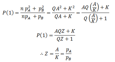
In summary, the generalized logistic form of P(t) is:
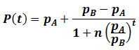
For any values of n, pA, pB, and t, both forms of P(t) give identical values. They are mathematically equivalent, although the above form is simpler and more convenient. Having found a simpler expression for P(t), we can find its inflexion point, the time at which the rate of average fitness increase is maximum. This is done by finding the second order derivative of P(t):
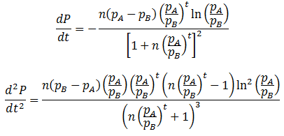
The inflexion point (tifx) occurs when its second derivative is equal to zero:
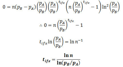
This equation corroborates what we would expect qualitatively. When n=1, the inflexion point occurs at t=0. Thus, the rate of change in the population’s average fitness is greatest when the instantaneous numbers of members in the fit and unfit groups are the same. Before this point the increase rate is limited by the small number of fit population and above it is limited by the small number of unfit population.
Also, the inflexion point does not exist when pB=pA. This is expected, as then there is really only one group and thus the average fitness would be constant. Inflexion only occurs at positive time when pB>pA and n>1, or n<1 and pA>pB. In other words, when there are initially more unfit organisms than fit organisms.
Lastly, this equation elucidates the specific relationship between the relative fitness of two phenotypes and the rate at which their frequencies in the population change. The tifx values can be taken as a measure of how quickly the population changes, a smaller value indicating a faster rate of change. Therefore, the rate increases with the logarithm of the phenotypes’ relative difference in fitness.
Generalizing the binary model
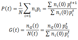
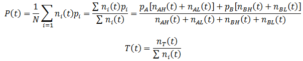
The previously characterized scenario, where there is evolutionary selection between only two possible phenotypes is not a very likely one. In real biological systems there are often many possible variants of a phenotype, some are controlled by so many different genes that a continuous range is observed. It is therefore of interest to consider the general case, when there is more than just two possible phenotypes of a particular trait. The mathematical treatment of this situation is the same as that of the binary system, we merely need to include additional terms for each phenotype that exists. The average fitness (P) and the proportion of a given phenotype (G) can be expressed as:
Note that when we add additional phenotypes to these equations we generally get much more complicated functions that can no longer be modeled as simple logistic curves.
A model for single mutations
So far, we have assumed that each organism reproduces to give rise to more of itself. However, mutation is an essential aspect of evolution and should not be overlooked. Suppose that organisms can have the A or B for phenotype for a particular trait, as before. But these organisms now have a second trait, their mutation probability (M), which can be high (H) or low (L). There are four possible kinds of organism: AH, AL, BH, and BL. When organisms reproduce, there is a probability of M that a mutation will occur: the offspring’s phenotype for A/B will be the opposite of the parent’s. Thus for this model mutations can only interconvert between the pairs AH/BH or AL/BL. To model this system fully, equations for the number (n) of each of the four organism types as a function of time must be developed. Mutation complicates the calculations; it is now simplest to define the number of organisms of each class recursively, allowing n(t) to be calculated incrementally. We can start with a similar form to the previously used equations for n(t), but now defining it in terms of discrete time increments:
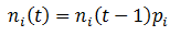
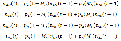
That is, the number of organism in the class increases/decreases each time increment by a factor of their fitness (p). This equation does not yet consider the effects of mutation however, so it is necessary to modify it. A fraction of 1-M of a given organism type will reproduce without mutation, thus this portion of the group can be treated with the above equation. The remaining M fraction undergo mutation, meaning their offspring are of the opposite phenotype (A/B). However, the parental mutation rate is conserved in the offspring. Thus a fraction of M class AL organisms will give rise to BL offspring for instance, while the other 1 – M fraction of the offspring will be AL. Mathematically, we can write this as:
We can follow the average fitness as before, substituting the above equations for the n(t) terms:
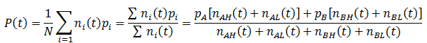
The fraction of any trait such as A, B, H, or L can be calculated by simply taking the ratio of the number of organisms with that trait (nT) to the total number as always. In general, the fraction a trait (T) is given by:
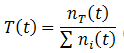
I performed the calculations using these equations with the parameters:
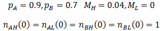
The results are plotted below, showing the frequency of phenotype A, (A), high mutation rate (H), and average fitness (P) as a function of time.
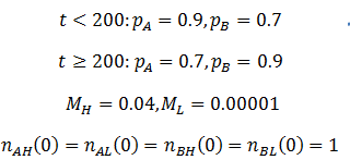
As we would expect the A phenotype outcompetes the B phenotype since its fitness is higher (p=0.9 vs 0.7), thus the fraction of phenotype A in the population approaches unity. However, the frequency of high mutation organisms decreases with time. In this case, mutation interferes with the selection of the most fit organisms. At high mutation rate there is lower correspondence between the traits of the parent and offspring. For instance, phenotype A organisms have a greater tendency to produce phenotype B organisms even though they are less fit. Mutation therefore decreases the speed and extent to which the more competitive phenotype can out-compete the other. This result may initially seem to contradict the commonly understood idea that mutation is important for evolution. However, an assumption that I had made implicitly in the models developed so far is that which phenotype is most fit is constant. Real biological systems are often subjected to changing conditions and environments though. Thus, the importance of mutation can be more fairly appraised under variable environmental conditions. In terms of the model, this means making the fitness values of phenotypes A and B a function of time. Suppose that their respective fitnesses are constant for a period of time, then there is a sudden environmental change which causes them to invert. I performed the simulation again with the parameters that follow. The results are plotted in the figure below.
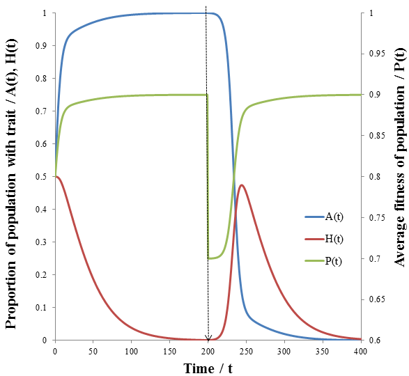
The dashed line indicates the time of the environmental change. At this point, almost all of the population is phenotype A, though suddenly phenotype B is now more fit. There are almost no organisms with phenotype B left, so the high mutation group has a substantial advantage over the low mutation group. The mutation-prone AH organisms produce a larger portion of phenotype B offspring than the AL organisms. This allows the high mutation group to recover faster from the environmental change and so the high mutation rate trait is selected for: the proportion of these trait increases dramatically following the environmental change. However, afterwards the environment is stable again and so the low mutation group out-competes the high mutation group eventually as in the previous case considered. It follows that for high mutation rate to be constantly selected for we require a constantly changing environment. I simulated this by periodically switching which phenotype produced the greatest fitness at 20 time unit intervals as follows:
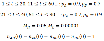
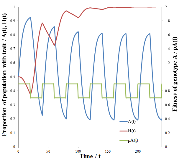
As predicted, a higher level of mutation is advantageous under constantly changing environmental conditions: the high mutation group entirely out-competes the low mutation group after a few cycles of variation. A higher rate of mutation allows the population to respond more rapidly to environmental changes. However, we would still expect too much mutation to have detrimental effects, even in a periodically changing environment. At greater the rates of mutation there is lower correspondence between the parent’s and offspring’s traits, as discussed previously. This reduces the efficiency at which the more fit phenotype is selected. In the most extreme case the offspring’s phenotype is random (M=1). In this case it is independent of the parent’s, allowing no adaption of the population to the current environment to occur. Thus the optimum rate of mutation is somewhere between the two extremes, depending on the particular conditions. To test this prediction, I repeated the above simulation varying the mutation rate (MH) of the high mutation group. I kept all other parameter constant as they were in the previous simulation. The results are presented in the following figure.
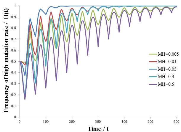
Indeed, a moderate mutation rate is optimum in a changing environment. When MH=0.05 the high mutation group out-competed the low mutation group the fastest. At mutation rates above or below this it took longer for the high mutation group to dominate the population. By trying different simulation parameters, I found that the optimum value varied with the frequency and size of the environmental changes.
Mutation rate as a mutable trait
The previous model made the simplifying assumption that only the trait A/B could mutate during reproduction, the rate of mutation itself was constant. This is not a realistic assumption, as mutation rate is surely influenced by heritable traits. Furthermore, it is easy to think of disadvantages of having a fixed mutation rate. A mutable mutation rate would make the population more able to respond to environmental change effectively. This advantage is important when the variability of the environment changes, such as from a highly variable environment (which trait is most fit, A or B, varies periodically) to a stable environment (the same trait is constantly most fit, suppose trait A). The AH/BH and the AL organism classes are most competitive in these respective environments. When mutation rate is fixed the high mutation group is unable to give rise to low mutation offspring. Thus, only the currently living AL organisms are available to out-compete the others. In contrast, when mutation rate is mutable, a fraction of the offspring of the abundant BH and AH organisms will be AL organisms. Thus the optimum class, AL, is able to out-compete the others faster, as a higher initial number of them are produced. Note that in the extreme case where we start with only AH/BH organisms, no AL organisms can be generated when mutation rate is not mutable.
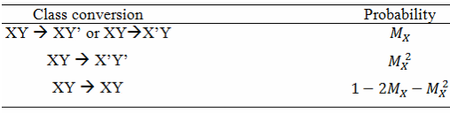
We still have four possible organism classes (AH, AL, BH, and BL). Mutation of the A/B phenotype and the mutation rate are independent. Now I define M as the absolute probability of single mutation of either of these traits. The resulting probabilities of all possible conversions are shown in the following table. I use XY to represent the organism class: X refers to H/L and Y represents A/B. Primes indicate a change in the indicated trait.
We still have four possible organism classes (AH, AL, BH, and BL). Mutation of the A/B phenotype and the mutation rate are independent. Now I define M as the absolute probability of single mutation of either of these traits. The resulting probabilities of all possible conversions are shown in the following table. I use XY to represent the organism class: X refers to H/L and Y represents A/B. Primes indicate a change in the indicated trait.
Mathematically, this means that we must calculate the number of organism in each class as follows:
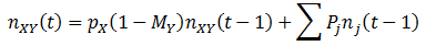
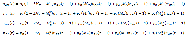
The summation is conducted for each of the other organism classes and P is the probability of the given conversion (see above table). Thus, for each organism classes, the equations are:
The equations used previously to calculate P(t) and the fraction of each trait (T) still apply:
Now that the math has been developed, we can return to the situation described above. That is, a highly variable environment changing (the most fit phenotype changes regularly) to a stable environment (where trait A is most fit). I predicted that AH/BH would out-compete the other organism classes during the variable phase, but the AL organisms would dominate when the environment becomes stable (at t>175). I did the calculations using the following parameters:
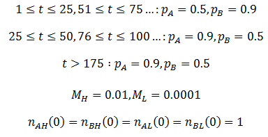
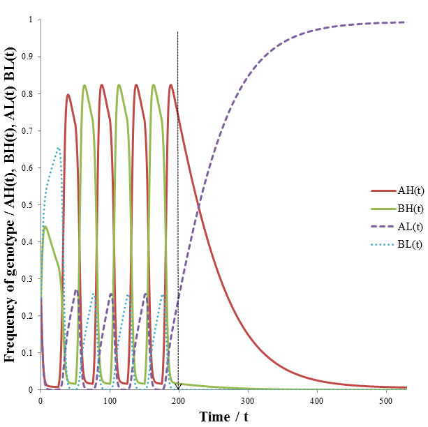
The line drawn indicates the time at which the cycle of variation ends. At t=200 during the cycle phenotype B would have become most fit. Instead, phenotype A now remains the most fit for the remaining duration of the simulation. The results are in excellent agreement with my predictions. Note that the AH and BH organisms dominant the population during the period of environmental variation. There are also some AL and BL organisms, some of these are produced each time increment by mutation. When the environment becomes stable the AL organisms out-compete the AH group. Having a high mutation rate becomes detrimental in a stable environment, as we have already seen in the former model. The advantage of allowing mutation rate itself to be mutable is evident from how quickly the AL organisms are able to dominant the population when the environment becomes stable at t=200. During the variable environment phase, AH and BH organisms are abundant. However, some of their offspring has the AL or BL phenotypes due to mutation. This means that is always a pool of AL/BL organisms available, even when high mutation rate is strongly selected for. Contrast this with the previous model, where after a period of variation the high mutation group eventually entirely out-competed the low mutation group. This difference allows a population with a mutable mutation rate to respond faster to changes in environmental variation. In the case of this simulation, we went from a variable to a stable environment. The mutable mutation rate gave the population a sufficient initial pool of AL organisms to quickly out-compete the AH organisms quickly when the environment suddenly became stable.
Genotype and sexual reproduction
The only source of variation between parents and offspring that I have examined so far is mutation. However, another important source of this is sexual reproduction. In order to model this though, the genotype of organisms must now be considered. I have modeled the competition of two phenotypes, A and B. Although this situation makes for a simple model, it is not very realistic. Real organisms have two copies of each gene (alleles), collectively making up their genotype. These alleles are the heritable elements, not the phenotype directly. Thus, I now will develop a model for the evolution of a population based on their genotypes. Imagine now for a particular gene there exists two alleles in the population, A and B. Organism can have two copies of one allele (homozygous, AA or BB) or a copy of each (heterozygous, AB). During sexual reproduction, there are six different combinations of genotypes possible for the mating organisms: AAxAA, AAxAB, AAxBB, ABxBB, ABxAB, and BBxBB.
The inheritance of the alleles from each parent are independent, thus it is easy to calculate the proportion of each genotype expected for in the offspring. This is traditionally shown as a Punnett square. For instance, for the mating of ABxAB:
The inheritance of the alleles from each parent are independent, thus it is easy to calculate the proportion of each genotype expected for in the offspring. This is traditionally shown as a Punnett square. For instance, for the mating of ABxAB:
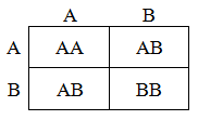
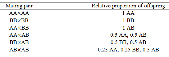
Thus, half of the offspring from this mating will have the genotype AB, a quarter will have AA, and the final quarter will have BB. In the following table the proportion of each genotype expected from each possible mating pair are summarized. These ratios are needed for the construction of the model.
In order to determine the fitness of each organism the effect of the genotype on the phenotype must be considered. Often, one allele is dominant and the other is recessive. For instance, if A is dominant and B is recessive, AA and AB would both have the phenotype associated with the A homozygote and only BB would have the B homozygote phenotype. Another possibility is co-dominance, where the A and B alleles both contribute to phenotype such that AB has a different phenotype than either AA or BB.
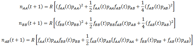
The fitness (p) of the organism class’s phenotype determines the proportion of them that reproduce successfully over a time increment (parental organisms are assumed to die after each time increment, leaving only offspring). The calculation of the amount of each genotype that are produced is complicated by how at any given time there may be different frequencies of organisms with each genotype in the population. I assume that mate selection is random (organisms do not show preference for mating partners based on genotype/phenotype). Thus, the probability of each of the above mating pairs are proportional to both the fitness values of each genotype and their frequencies (f) in the population. The number (n) of each genotype offspring produced can be found by summing the numbers produced by all possible crosses listed above. This is done over discrete time intervals as with the mutation models:
The fitness (p) of the organism class’s phenotype determines the proportion of them that reproduce successfully over a time increment (parental organisms are assumed to die after each time increment, leaving only offspring). The calculation of the amount of each genotype that are produced is complicated by how at any given time there may be different frequencies of organisms with each genotype in the population. I assume that mate selection is random (organisms do not show preference for mating partners based on genotype/phenotype). Thus, the probability of each of the above mating pairs are proportional to both the fitness values of each genotype and their frequencies (f) in the population. The number (n) of each genotype offspring produced can be found by summing the numbers produced by all possible crosses listed above. This is done over discrete time intervals as with the mutation models:
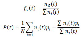
Where R is the reproductive factor, a value that reflects how many viable offspring are produced by reproduction. The frequencies of each genotype (fG) and average fitness (P) are calculated according to:
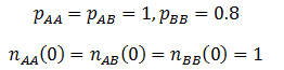
Note that like the carrying capacity term, we can ignore the R term since we are only concerned with relative ratios. Now that the model has been formulated, we can begin to study its properties. First, I looked at the case where the A allele is dominant to B and the AA/AB phenotype is more fit than the BB phenotype. The parameters were:
The frequency of each genotype are plotted as a function of time in the figure below.
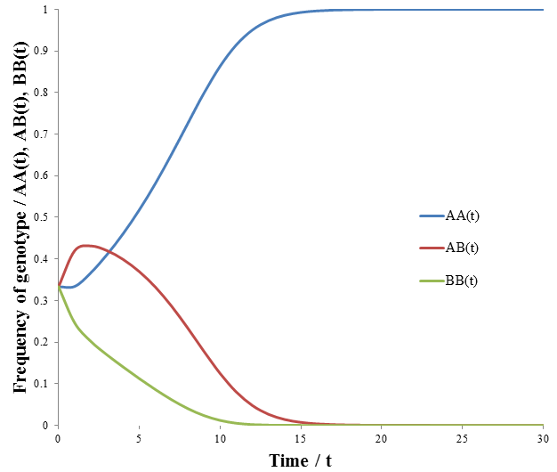
The AA genotype out-competes the others, becoming the sole genotype of the population eventually. It may surprise you that the AB genotype was out-competed, since it had the same fitness as the AA genotype. However, they differ in the offspring will can produce. A population of AA genotypes can give rise to only AA. Regardless of what genotype they mate with, the unfit BB genotype is not produced. In contrast, offspring of an AB will include the unfit BB genotype. The AA genotype produces more fit offspring, and thus proliferates more readily. This reveals that we must not only consider the fitness of the organism, but also of its offspring when evaluating a trait’s value.
Similar frequency profiles are obtained in the case where the A allele is recessive, but still the most fit. However, it is interesting to compare the rate at which the AA genotype out-competes the others. I simulated the recessive case using the following parameters:
Similar frequency profiles are obtained in the case where the A allele is recessive, but still the most fit. However, it is interesting to compare the rate at which the AA genotype out-competes the others. I simulated the recessive case using the following parameters:
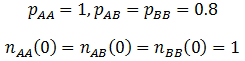
The frequency of the AA genotype as a function of time is plotted below for both cases:
Thus, when the A allele is recessive there is stronger selection of it, it dominants the population faster. There result can be rationalized quite easily. When the A allele is dominant both the AA and the AB genotypes have greater odds of reproducing due to higher fitness. However, only the AA genotype has an advantage in the recessive case. The selection of the AA genotype is consequently more explicit.
Heterozygous advantage
Heterozygous advantage refers to the situation when the heterozygous genotype (AB) has greater fitness than either homozygous genotype (AA or BB). Interestingly, during sexual reproduction the AB genotype must give rise to AA and BB organisms. Even if the heterozygous state is most fit a population can stably contain at maximum 50% heterozygous organisms (recall that the ABxAB cross gives rise to 50% AB, 25% AA, and 25% AA genotypes). At equilibrium, we therefore expect the population to have some of each genotype. A popular real-world example of heterozygous advantage is sickle cell anemia. Having sickle-cell haemoglobin provides resistance to malaria. However, sickle-cell haemoglobin polymerizes under low-oxygen conditions, resulting in disease. Individuals heterozygous for sickle-cell haemoglobin have resistance to malaria but do not suffer the disease since 50% of their hemoglobin is normal. Thus, because of the high fitness of the heterozygote, the sickle-cell trait persists in regions with frequent malaria outbreaks, even though it causes disease in individuals homozygous for the trait. For instance, in equatorial Africa as much as 40% of the population are carriers of the trait.
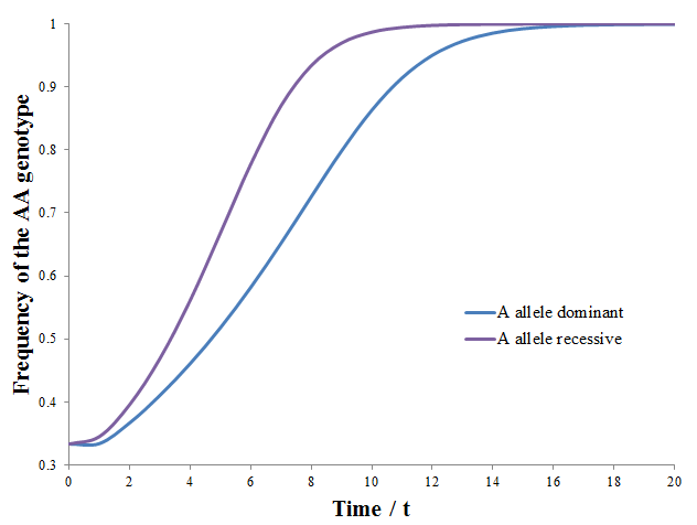
An interesting question results from this: what is the ideal proportion of each genotype in such a population, how is this affected by the relative fitness of each? It is tempting at first glance to think that since the heterozygous genotype is most fit the equilibrium ratio will favour a maximum amount of AB, 50%. However, my analysis shows the situation to be more complex than this, a supporting example follows. The figure below gives the frequencies of each genotype with respect to time calculated using following parameters:
An interesting question results from this: what is the ideal proportion of each genotype in such a population, how is this affected by the relative fitness of each? It is tempting at first glance to think that since the heterozygous genotype is most fit the equilibrium ratio will favour a maximum amount of AB, 50%. However, my analysis shows the situation to be more complex than this, a supporting example follows. The figure below gives the frequencies of each genotype with respect to time calculated using following parameters:
The population had the general behavior we had expected, heterozygote advantage resulted in an equilibrium where there is some of each genotype. However, the exact equilibrium frequencies of AA/BB and AB were 0.26047 and 0.47907 respectively. This is slightly different from the 0.25/0.5/0.25 ratio you might have expected. However, this deviation is expected if the matter is given further thought. Over each time increment 25% of the ABxAB reproductions that occur give rise to the AA genotype and another 25% to the BB genotype. If all of these organisms died/did not reproduced successfully (e.g. if pAA, pBB = 0), then at any given time there would only be 25% of the AA and 25% of the BB genotypes. However, if some do reproduce (pAA, pBB > 0), then some additional AA or BB offspring will be produced beyond the 25% from ABxAB reproduction. Since these are less fit than the AB genotype, it is tempting to think that these offspring will be out-competed and the population should tend towards the 0.25/0.5/0.25 ratio. However, remember that each time increment another 25% of AA and 25% of BB genotypes are produced from ABxAB reproductions. Thus a small additional amount of AA and BB organisms are expected to persist beyond the 25% expected from ABxAB reproductions alone. The exact ratio at equilibrium would be a function of the relative fitness of each genotype. Despite this, deriving a simple algebraic expression to predict this ratio has proven difficult. It could be that the complexity of the system does not permit a simple algebraic solution, perhaps the only way to calculate the ratio is to simply perform the simulation.
In order to test the validity of my explanation above for the 0.26047/0.47907/0.26047 AA:AB:BB ratio, I did the simulations again for different fitness values of each genotype. The results follow in the table below.
In order to test the validity of my explanation above for the 0.26047/0.47907/0.26047 AA:AB:BB ratio, I did the simulations again for different fitness values of each genotype. The results follow in the table below.
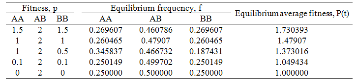
A prediction of my explanation follows: when the fitness of the AA and BB genotypes are decreased relative to that of the AB genotype, the genotypic ratio at equilibrium should approach the 0.25/0.5/0.25 ratio. This is because the AA and BB organisms would have a lower tendency to reproduce successfully and thus cause a smaller deviation from this ratio. The data above show this trend, validating my explanation. In the extreme case where pAA=pBB=0, the ratio of 0.25/0.5/0.25 is obtained exactly as we would expect.
Interestingly, upon trying a variety of fitness values I found that the heterozygous genotype having greatest fitness did not guarantee that the population would contain a mix of genotypes at equilibrium. Instead for any set of fitness values where pAB > pAA, pBB there exists many combinations of pAA and pBB values such that the heterozygotes are out-competed by one of the homozygous genotypes. That is, the condition pAB > pAA, pBB is necessary, but not sufficient for a heterozygous-containing equilibrium to result. Observe below, where I used the parameters:
Interestingly, upon trying a variety of fitness values I found that the heterozygous genotype having greatest fitness did not guarantee that the population would contain a mix of genotypes at equilibrium. Instead for any set of fitness values where pAB > pAA, pBB there exists many combinations of pAA and pBB values such that the heterozygotes are out-competed by one of the homozygous genotypes. That is, the condition pAB > pAA, pBB is necessary, but not sufficient for a heterozygous-containing equilibrium to result. Observe below, where I used the parameters:
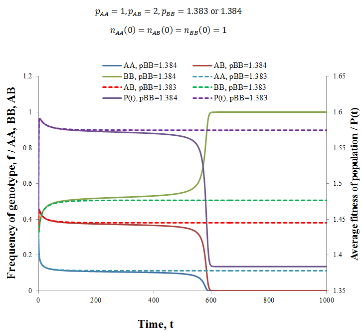
Compare the solid lines (pBB=1.1384) to their corresponding dashed lines (pB=1.1383), note the vastly different outcomes resulting from a difference in pBB values of only 0.001! When pBB=1.383 an equilibrium is reached containing some of each genotype, while when pBB=1.384 the BB genotype out-competes the others and dominates the population. In fact, holding the other fitness values constant, any pBB value > 1.383 produces this result. Thus, there appears to be some critical threshold below which a stable equilibrium containing the heterozygote exists. Despite considerable effort, deriving an algebraic expression for this turning point in terms of the fitness values has proven difficult. Like with the equilibrium ratios, it is likely that the complexity of the system does not allow for a simple algebraic solution. Nevertheless, I can suggest a qualitative explanation for the effect. Refer back to the last table where I gave the equilibrium frequencies and average fitnesses for a variety of genotype fitness values. Notice that for each case average fitness at equilibrium is greater than the fitness of either homozygote alone. This explains why this equilibrium containing the homozygote is favourable; the fitness is greater than if the population consisted of either homozygote alone. I therefore propose that the turning point observed (pBB=1.384) occurs when the fitness of the BB genotype alone is greater than the average fitness that could be stably achieved with a heterozygote/homozygote equilibrium. In summary, there appears to be values of pAA and pBB for any pAB > pAA, pBB such that a population of a single homozygote is obtained at equilibrium.
I included the average fitness in this figure because, interestingly, it actually decreases with time initially. This is the first case in this entire investigation where we have seen average fitness decreasing with time. This may seem to contradict what I presented as the basis of evolution, that differential selection of more fit organisms gives rise to increasing fitness in the population over time. However, this is really just a result of the starting conditions chosen and the properties of co-dominant genes. If the population starts at a position far from equilibrium, but more fit than at equilibrium, its fitness must decrease until equilibrium is reached. For instance, in a more extreme case imagine starting with only heterozygous (AB) organisms. At most, they can sexually reproduce to give offspring that are 50% AB, thus the amount of AB would have to decrease even if the AB genotype confers greatest fitness. Therefore there is a distinction between stability and fitness. We can thus amend the previous statement: populations approach the maximum average fitness that can be attained stably.
I included the average fitness in this figure because, interestingly, it actually decreases with time initially. This is the first case in this entire investigation where we have seen average fitness decreasing with time. This may seem to contradict what I presented as the basis of evolution, that differential selection of more fit organisms gives rise to increasing fitness in the population over time. However, this is really just a result of the starting conditions chosen and the properties of co-dominant genes. If the population starts at a position far from equilibrium, but more fit than at equilibrium, its fitness must decrease until equilibrium is reached. For instance, in a more extreme case imagine starting with only heterozygous (AB) organisms. At most, they can sexually reproduce to give offspring that are 50% AB, thus the amount of AB would have to decrease even if the AB genotype confers greatest fitness. Therefore there is a distinction between stability and fitness. We can thus amend the previous statement: populations approach the maximum average fitness that can be attained stably.
Conclusion
Using relatively simple models, I have been able to verify a variety of accepted aspects of evolutionary theory, as well as elucidate some new details:
--The frequency profiles of two competing traits in a population follow a logistic curve in a stable environment.
--The rate at which the frequency of heritable traits in a population change is greatest when the frequencies of the competing traits are equal.
--The time required for one trait to out-compete another varies with the logarithm of the traits’ relative fitness values.
--Mutation is advantageous and thus selected for during times of environmental change, but is detrimental when the environment is stable.
--For any population there exists an optimum mutation rate based on the frequency and size of environmental changes.
--Having a mutable mutation rate is beneficial when the variability of the environment changes.
--In addition to the direct fitness conferred to an organism by a particular trait, the resulting fitness of its offspring must also be considered when appraising its overall competitiveness.
--The selection of a fit recessive allele occurs faster than for a dominant allele.
--If a homozygous genotype is more fit than the other genotypes, it will dominant the population at equilibrium.
--Heterozygous advantage can result in an equilibrium mixture of each genotype, where the ratio depends on the relative fitness values of the genotypes. However, the heterozygote having highest fitness alone does not guarantee that such equilibrium will occur; there is also dependence on the homozygotes’ fitness values.
Mathematical modelling can be a useful check of our assumptions and reasoning, to verify they made the predictions that we think they do. It is reassuring that my models, although relatively simplistic, corroborated many predictions of evolutionary theory and population dynamics.
I argued at the start of this article that modelling could also be used to address questions that are not testable experimentally. A good demonstration of this is my study of heterozygous advantage. This phenomena, the heterozygous state having greater fitness than either allele alone, is sometimes used to help account for genetic variation in populations. Indeed, my simulation results predicted that heterozygous advantage could maintain genetic variation by allowing a mixture of genotypes at equilibrium. However, I was also able to show that heterozygous advantage alone did not always produce such a mixture. Though this result was very feasible to show mathematically, it would be challenging to demonstrate experimentally. Unlike with real organisms, when running a simulation you have full knowledge and control of the fitness values assigned to each genotype.
The simplicity of the models I have presented was convenient when performing the calculations; I could do them using Microsoft Excel. However, it limited the types of questions that I could study. For instance, I assumed the population was infinite to simplify the model. There are many evolutionarily important consequences of smaller population sizes though, such as genetic drift. Furthermore, I studied cases where there are only a few discrete phenotypes in the population. In contrast, for real populations many phenotypes are quantitative, they vary over a continuous spectrum. It would be interesting to study the dynamics of a population with several quantitative traits. In this case, fitness would be a complex function of all traits possessed by the organism, as well as the state of the environment. This raises an intriguing issue that I have not been able to examine through my current models: local versus global maxima of evolutionary fitness. We can imagine a fitness landscape, a surface that visually relates the fitness of an organism to all of its traits and the current environment. Mutation and genetic recombination from sexual reproduction allow a population’s members to transverse the fitness landscape, moving towards a fitness maximum. However, depends on the shape of the landscape, this may not be the global maximum. In a future article, I will study how evolving populations move through fitness landscapes. The problem of local minima is of particular interest to me, including what conditions and through what mechanisms populations are able to find the global maximum. The problem of finding global maxima has applications to a variety of fields, not just evolutionary biology. Indeed, algorithms inspired by evolution are often used to search for solutions to optimization problems. Elucidating how the problem can be solved in the case of evolution may provide new insights and strategies to solving it in the general case. Unfortunately, the complexity of the model needed for this a simulation is beyond what is reasonable to do in Excel. It is possible to design a computer program to do the calculations though, the develop of such a model may be the topic of a future article.
 RSS Feed