In my previous article on the mathematical modeling of evolution I developed several models to quantitatively examine and observe various aspects of evolution. Here I extend this work, examining how mutation rate affects the equilibrium state of an evolving population.
In the simplest model I previously developed, each organism in a large population had one of two possible phenotypes, A or B (the binary system). Reproduction was exclusively asexual and there was no mutation. This means that all organisms of a given phenotype could give rise only to offspring of the same phenotype. I recommend reviewing my previous article, but here I will summarize the main results:
In the simplest model I previously developed, each organism in a large population had one of two possible phenotypes, A or B (the binary system). Reproduction was exclusively asexual and there was no mutation. This means that all organisms of a given phenotype could give rise only to offspring of the same phenotype. I recommend reviewing my previous article, but here I will summarize the main results:
Here t refers to time, nA and nB refer to the initial relative number of A and B phenotype organisms, pA and pB refer to their relative fitness, A(t) and B(t) represents the average fraction of each phenotype in the population, and P(t) refers to the average fitness of the population.
The equilibrium behavior of this type of system is easy to predict: as long as one of the phenotypes confers greater fitness, it will eventually entirely out-compete the other. That is, the equilibrium state will always be a population composed entirely of the more fit phenotype. While I examined some affects of mutation rate on evolution in my previous article, I did not investigate its affect on the equilibrium state of the population. Thus, in this article I will elucidate this relationship.
The equilibrium behavior of this type of system is easy to predict: as long as one of the phenotypes confers greater fitness, it will eventually entirely out-compete the other. That is, the equilibrium state will always be a population composed entirely of the more fit phenotype. While I examined some affects of mutation rate on evolution in my previous article, I did not investigate its affect on the equilibrium state of the population. Thus, in this article I will elucidate this relationship.
A model for population evolution with mutation
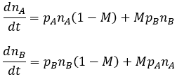
To keep the mathematics feasible I develop this model starting with the previously mentioned binary system. Suppose that all members of a large population have the same probability of mutation (M). If a mutation occurs, the parent gives rise to offspring of the opposite phenotype. The other 1 – M portion of offspring are born with the same phenotype as the parent. The phenotypes A and B confer fitnesses pA and pB to the organism respectively. The fitness of an organism is a relative measure of its survival and reproductive success. For clarity, I always define A as the more fit phenotype. We can thus calculate the relative amount of phenotype A (nA) and phenotype B (nB) in the population recursively as follows:
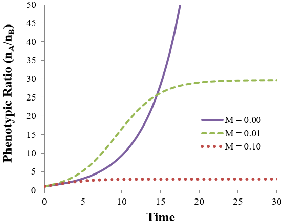
The consequences of adding mutation may not be obvious from these equations. I therefore plot the outcomes at different mutations rate below, using the parameters: nA=nB=1, pA=1, and pB=0.7.
If the mutation rate is zero (M=0) the ratio of phenotype A to B increases exponentially towards infinity. Since phenotype A is more fit than phenotype B, the equilibrium state consists of 100% phenotype A. However, if the mutation rate is nonzero (M > 0), the population moves towards some equilibrium ratio between the phenotypes, as seen by the plateaus in the figure above. A higher mutation rate results in a lower the phenotypic ratio of A to B. This can be understood qualitatively: a higher mutation rate means that there is less correlation between the phenotype of the parent and the offspring. Even though phenotype A is more fit, some phenotype B organisms will always be produced through mutations. A higher mutation rate leads to more B offspring being produced each generation, decreasing the equilibrium ratio of phenotype A to B (compare the equilibrium plateaus of the M=0.01 and M=0.1 lines).
The relationship between mutation rate and population equilibrium state
While we qualitatively understand how mutation rate affects the population equilibrium, I was interested in a more quantitative prospective. I wanted to calculate the equilibrium ratio of A to B as a function of pA, pB, and M. Simulation of the population given any set of these parameters allowed the true equilibrium ratios to be determined. I did this for many combinations of these values and found their relationship to be surprisingly complex. Deriving an equation for it through first principles proved challenging due to the intricate, iterative nature of the equilibrium: each subsequent generation depends on the composition of the previous generation. Developing an algebraic equation for the composition of the nth generation was not feasible. Nevertheless, this is not required if we are only interested in the population’s composition at equilibrium. The defining feature of the equilibrium state is that the ratio of A to B phenotype in the population is constant. This requires that the relative rate of change in the number of A and B phenotype organisms be equal.
The rates of change in the relative frequency of phenotype A and B are given by:
The rates of change in the relative frequency of phenotype A and B are given by:
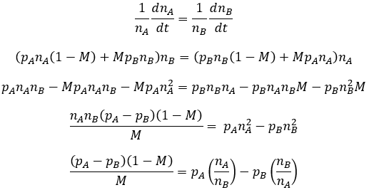
At equilibrium, the phenotypic ratio of the population is constant. This means that the relative rates of change for both phenotypes are equal. Mathematically, their normalized derivatives are required to be equal:
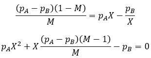
Now let X represent nA/nB:
This is a quadratic whose roots can be found according to the quadratic equation.
Satisfyingly, this equation has accurately predicted the equilibrium ratio for all simulated populations I have checked it against. For instance, consider the two cases plotted in the earlier figure with M=0.1 or 0.01 at pA=1, and pB=0.7. Calculating the equilibrium ratios we accurately predict nA/nB = 2.94 and 29.72 respectively.
Examining the terms in this equation, notice that mutation rate (M) always occurs as (1-M)/M. It is interesting to consider the meaning and significance of this. This term gives the ratio of unmutated to mutated offspring a parent will have. For instance, if the mutation rate is 10%, 9 unmutated offspring are produced for every mutated one. Correspondingly, we have (1-M)/M=9. I therefore define this term as conservation (C) since it quantifies how conserved a trait is from parent to offspring.
Examining the terms in this equation, notice that mutation rate (M) always occurs as (1-M)/M. It is interesting to consider the meaning and significance of this. This term gives the ratio of unmutated to mutated offspring a parent will have. For instance, if the mutation rate is 10%, 9 unmutated offspring are produced for every mutated one. Correspondingly, we have (1-M)/M=9. I therefore define this term as conservation (C) since it quantifies how conserved a trait is from parent to offspring.
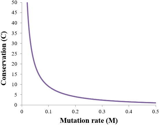
To clarify the relationship between conservation and mutation rate, I plot it from M = 0.01 to 0.5 below.
At M=0.5, all parents give 1:1 mixtures of A and B phenotype offspring, giving a minimum conservation of 1. As mutation rate is decreased toward 0, conservation tends to infinity as nearly all offspring share the phenotype of their parents.
The conservation term allows us to rewrite the equilibrium equation in a simpler form.
The conservation term allows us to rewrite the equilibrium equation in a simpler form.
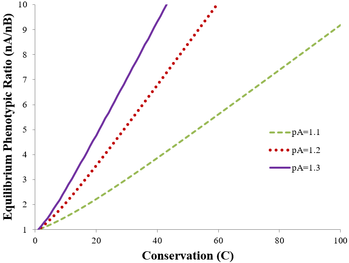
We can gain insight about the effect of mutation rate on evolutionary equilibrium by graphically examining this equation. Below I evaluate it at pB = 1 and pA = 1.1, 1.2, or 1.3.
The equilibrium ratio increases to favor the more fit phenotype both as its relative fitness is increased (increasing pA) or conservation is increased (decreasing mutation rate). The equilibrium ratio is linear with conservation at high conservation values, but deviates at low values. Mathematically, this is due to the quadratic nature of the equation. However, this feature can also be understood qualitatively. At high conservation the population is overwhelmingly composed of the more fit phenotype, limiting the confounding iterative contribution of mutant offspring on the equilibrium ratio. In contrast, low conservation results in an appreciable pool of mutant offspring whose iterative mutant and non-mutant offspring add complexity to the equilibrium phenotypic ratio.
Limiting cases of the mutation-equilibrium equation
A final approach to gain insight about this system is to consider special limiting cases of the equation. A few are presented here.
pB = 0
Suppose a mutant phenotype is nonlethal but renders an organism entirely unable to reproduce. In my equations that would be indicated by pB = 0. In this case the equilibrium ratio simplifies greatly to the unmutated to mutated ratio (by definition, the conservation).
pB = 0
Suppose a mutant phenotype is nonlethal but renders an organism entirely unable to reproduce. In my equations that would be indicated by pB = 0. In this case the equilibrium ratio simplifies greatly to the unmutated to mutated ratio (by definition, the conservation).
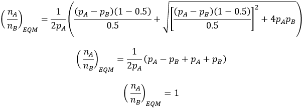
M = 0.5
This extreme case represents the maximum mutation rate, where offspring phenotype is entirely unrelated to that of the parents. As we intuitively expect, this gives rise to 1:1 phenotypic ratio at equilibrium, independent of their relative fitness values.
This extreme case represents the maximum mutation rate, where offspring phenotype is entirely unrelated to that of the parents. As we intuitively expect, this gives rise to 1:1 phenotypic ratio at equilibrium, independent of their relative fitness values.
M = 0
When no mutation is possible, the situation simplifies to the binary model given in my previous article. Here we obtain a homogeneous population of the more fit phenotype at equilibrium, with the phenotypic ratio tending toward infinity.
When no mutation is possible, the situation simplifies to the binary model given in my previous article. Here we obtain a homogeneous population of the more fit phenotype at equilibrium, with the phenotypic ratio tending toward infinity.







 RSS Feed