In this article, I develop a simplistic mathematical model for the growth of hair. Consider a population of N hairs. Different hairs may have different length (l). Over discrete time intervals (t) hairs may either grow by a constant length (k) or fall out, resetting their length to zero. Each hair has the same probability of growing instead of falling out over a given time interval (p). Thus we can describe the length of a given hair as a function of time as:
Where G(p) is a function which randomly returns either zero or one based on the value of p. It returns one a proportion of p times and zero a proportion of 1-p. In order to actually achieve this, the If() and Rand() functions can be used in Excel:
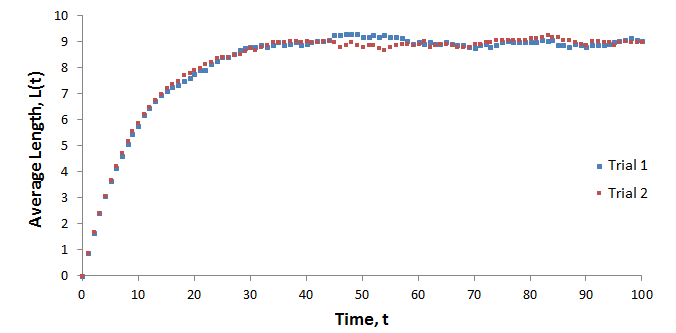
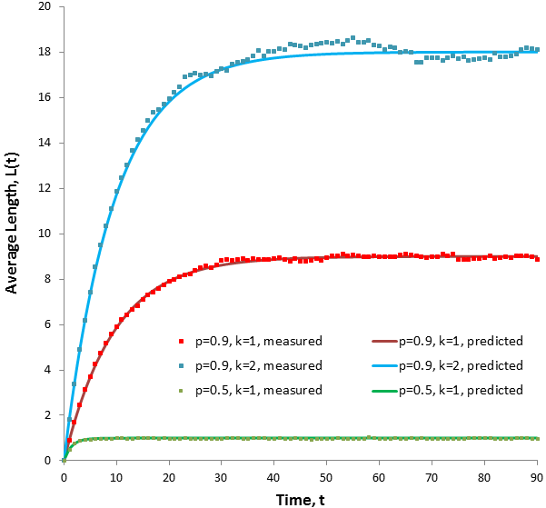
I used the l(t) function above in Excel to calculate the lengths of individual hairs (N=4500) and computed the average (L) as a function of time. The initial length of each hair was zero, p=0.9, and k=1. The results for two trials performed are shown below.
Both curves follow the same trend and plateau at an average length of 9. The variation seen in the plateaus are the result of random fluctuations due to the limited sample size. An infinite population of hairs would have no variation in its plateau. It is intuitive that the average length eventually becomes constant. Equilibrium is reached such that the rate at which average length increases due to hair growth and the rate at which it decreases due to hairs falling out are equal.
My goal is to develop simple equations to describe the curves that result from these calculations. The typical person has of the order of a hundred thousand hairs on their head. Hence by the Law of Large Numbers the probabilistically expected result will be identical to the actual result. Thus, I will model this situation by computing the probabilistically expected results.
My goal is to develop simple equations to describe the curves that result from these calculations. The typical person has of the order of a hundred thousand hairs on their head. Hence by the Law of Large Numbers the probabilistically expected result will be identical to the actual result. Thus, I will model this situation by computing the probabilistically expected results.
Average hair length at equilibrium
First I will develop an expression for the maximum average length (M), the average length at which the curve plateaus. The average hair length is given by summing the products of each length and its probability:
In order to evaluate this sum we must therefore find the probability associated with each length. To think about this it is useful to consider a single strand of hair. It is easy to calculate the probability of the strand not falling out up to a given time interval. By the definition of p, this probability is p at t=1, p^2 at t=2, and so forth. Note that the probability of the strand being intact at t=0 is defined as 1. However, these values are not quite the true probabilities of the hair being in a particular state. This should be obvious from how the sum of the terms exceeds unity. These are relative probabilities, proportional to the absolute probabilities we seek. We must consider how the hairs are partitioned between the full spectrum of possible length states. We can get the probability of each length state if we divide this series by the sum of probability terms to normalize the distribution:
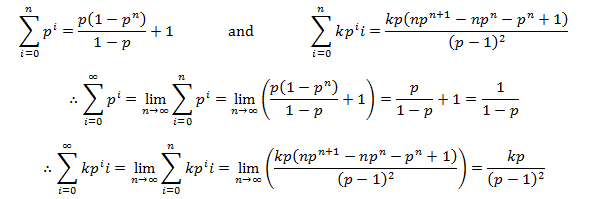
The initial length term was dropped because the initial length of hair before growth is zero. To evaluate these infinite sums we must utilize some results from the mathematics of sequences and series:
Now we can use these results with the definition of M to develop a simpler expression for average length at equilibrium:
Average hair length as a function of time
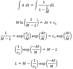
Since the average length-time curves plateau, we know the rate of change of average length with respect to time must decrease as L approaches M, with dL/dt=0 when L=M. The differential equation can therefore be written as:
Where A is some unknown constant of proportionality to be determined. Now solving the differential:
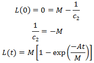
We had assumed that the initial length of each hair is zero, thus L(0)=0.
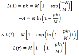
We can deduce the value of L(1) quite easily. All hairs initially have a length of zero. Over the first time interval a fraction of p hairs will grow a length k while all others remain with a length of zero. Thus L(1)=pk. This allows us to determine the value of A:
We can simplify this by substituting the equation for M derived above:
We finally have a general equation which gives the average length of hair at any time. Note that L(t) approaches M as t becomes large, as we would expect. We can verify the accuracy of this expression by comparing its results to the results obtained by simulating the length of a populations of hairs (N=4500). This was calculated as I described at the beginning of the article.
Note the excellent agreement between the measured results and those predicted by the model. As before, the measured values fluctuate slightly due to the limited sample size. Increasing the value of k increases the length at equilibrium but not the rate at which equilibrium is approached. At lower values of p the equilibrium length is lower, but equilibrium is reached faster.
At what time is equilibrium reached?
I have spoken about the properties of the system before and after equilibrium is reached. You might be wondering when exactly this is achieved. Unfortunately, this question does not have a simple answer as in principle it can only be fully reached after infinite time. However, in practice there are no discernible differences between a system very close to equilibrium and actually at equilibrium. To examine this quantitatively we can look at the average length as a fraction (f) of M. We use this to calculate the time (tf) needed for the length to reach a given fraction of M:
The value tf measures how quickly the system approaches equilibrium. As p increases the magnitude of ln p decreases and so the system takes longer to reach equilibrium. This is intuitive: hair which falls out less frequently would have a longer equilibrium length and so requires more time to grow to this length.
The distribution of hair lengths at equilibrium
It is worth noting that what I have been calculating, the average hair length, is different then what we normally think as the length of one’s hair. The visually apparent length is the length of the longest hairs. Many people have relatively short hair which is obviously well below the equilibrium length. The equilibrium length would be the maximum length achievable, obtained by never cutting one’s hair.
When thinking about the visually apparent length it is more useful to instead consider the distribution of lengths seen in the population of hairs. The numbers of hairs in each length state follow an exponential decay curve as the length of the state increases. This follows from what I had already shown regarding the probability of each length state earlier. For simplicity, let q be the complement of p: q=1-p.
First, I will derive an equation for the number of hairs in each length state when the system has reached equilibrium [i.e. L(t)=M]. The state i=0 has a length of 0. Recall that in a given time interval all hairs have a probability of q of falling out, of switching to the i=0 state. Note that this applies even to the i=0 state itself, a proportion of q of the hairs in the i=0 state will stay in this state over a given time interval. Thus the number of hairs in this state will be Nq, where N is the total number of hairs. Now consider the i=1 state. A proportion of p of the Nq hairs at i=0 will grow to the i=1 state. We needn’t consider the number of hairs previously occupying this state, as all either grow to the i=2 state or fall out and return to the i=0 state. Thus the number of hairs at the i=1 state are Nqp. This logic can be applied again to show that there are Nqp^2 in the i=2 state, Nqp^3 in the i=3 state, and so forth. In general:
An implication of this equation is that hair populations with higher p values have broader size distributions. In fact, this is why greater p values give rise to greater equilibrium average length. A higher p value means that the hair has a lower tendency to fall out and thus can grow longer.
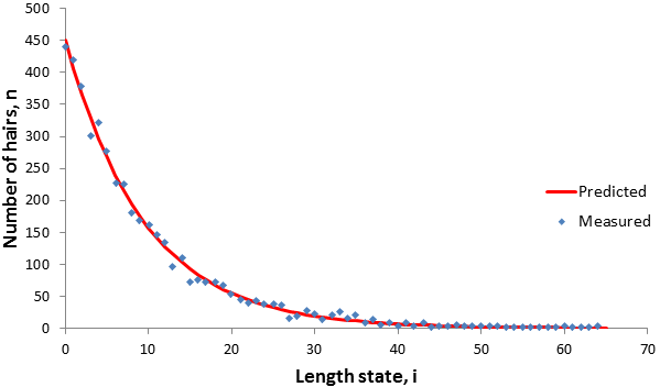
This model is consistent with the distribution I observe in simulated data. For instance, at equilibrium with N=4500 and p=0.9:
This model is consistent with the distribution I observe in simulated data. For instance, at equilibrium with N=4500 and p=0.9:
The distribution of hair lengths as a function of time
Remember that the above treatment was for when the system is at equilibrium. The situation becomes more complicated at earlier times before this. Since all hairs are starting from the i=0 state the time elapsed can limit the states accessible to the population. During each time interval some hairs can transition to a greater length state. For instance, at t=0 all hairs are in the i=0 state. At t=1 some hairs can occupy the i=1 state, at t=2 the i=2 state becomes available, and so forth. In general, the time gives the maximum i value allowed. For i values below t though, we can calculate the number of hairs in each state as we did when the system was at equilibrium. Note that the logic used to derive the n(i) equation did not really require equilibrium, only that i < t.
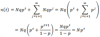
However, the i=t state is the highest accessible length state to the population. Here we must consider all hairs which transiently reached this state. We needn’t worry about the number which will leave in this iteration since there are no hairs initially occupying the state. Thus, the number is simply Np^t.
Should this argument not convince you, here is an alternative way of demonstrating this. We can consider two contributions to the number of hairs in the state i=t. Firstly, the normal Nqp^i term, but also the sum of all hairs which at later time will further distribute themselves among the higher length states at equilibrium:
Any length state with i>t cannot be occupied. Growth occurs incrementally so the longest available state is at i=t. Therefore n(i)=0 for all i>t. The full distribution can now be summarized as a piecewise function:
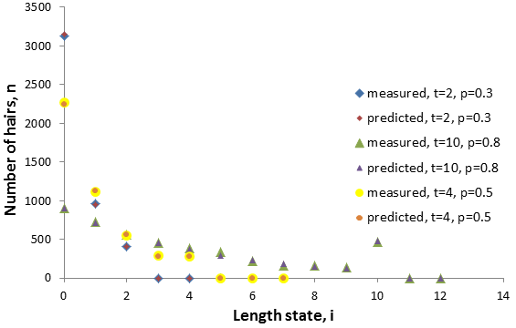
The figure below compares the model’s results for a few cases compared to those from the simulation (N=4500), they are in good agreement.
The behavior of the equation around i=t is interesting and worth paying special attention to. In particular, consider n(t-1) and n(t). We can compare the size of these terms by evaluating their ratio:
The n(t) term is larger than the n(t-1) term for p>0.5, smaller for p<0.5, and equal when p=0.5. These predictions are verified in the figure above. Thus, the p value determines the shape of the distribution around i=t.
The size of the peak when p>0.5 would of course increase with p, and vice versa for when p<0.5. In the case of human hair, recall that the number of hairs of a typical person is of the order of 10^5. A generous estimate for the number of hairs falling out per day is 100. Thus the p value would be of the order of 0.999 per day. Also, as I have argued before, the typical person’s hair is far below its equilibrium length. Therefore, the equation implies that typical human hair has a large peak in the distribution at the maximum length state, i=t. In other words, the majority of a typical person's hairs have the same length, with very few having shorter lengths. Upon inspecting your own head you will likely notice that most of your hairs have roughly the same length. Of course this illustration is complicated by unequal cutting of different regions during a haircut, but this works well focusing locally on a small region.
The intended application of the model I have developed is hair growth. However, it also applies to a wide variety of other situations, any which satisfy the assumptions made by the model. For instance, my results that could be applied to the heights of trees in a forest. The model would require that each tree cut down is replanted and that the selection of trees is independent of their height. Small modifications to the model could be done so that it more appropriately fits other situations. In the case of a forest, we may want to add a factor to make the cutting of trees biased towards taller ones, for instance.











 RSS Feed