A fundamental idea in finance is the time value of money: money now is worth more now than money later. Mathematically, this reality is described by the interest rate. The value of money in the present and future are related by the accumulation function:

Where A(t) is the future value, P is the initial principle, i is the interest rate, and t in the time in years.
In this equation (simple interest), the earned interest on the initial principle is not re-invested to earn additional interest, so the future value grows linearly with time. For instance, a principle of $100 at an interest rate of 10% would earn $10/year. Another possibility, however, is for these returns to be re-invested to increase the rate of accumulation. In the previous scenario, suppose the $10 earned each year is also invested at 10% interest annually. This scenario is called annual compounding:
In this equation (simple interest), the earned interest on the initial principle is not re-invested to earn additional interest, so the future value grows linearly with time. For instance, a principle of $100 at an interest rate of 10% would earn $10/year. Another possibility, however, is for these returns to be re-invested to increase the rate of accumulation. In the previous scenario, suppose the $10 earned each year is also invested at 10% interest annually. This scenario is called annual compounding:

Now the accumulation function grows exponentially with time. Alternatively, the compounding can be done multiple times per year (periodic compounding):

Where A is the final accumulated value, P is the principle, i is the interest rate, n is the number of times compounded per year, t is the time in years.
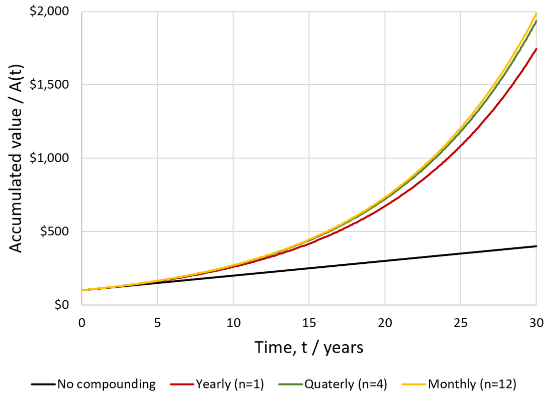
To explore the consequences of compounding, I compare below the growth of $100 invested at 10% interest under simple interest versus annual, quarterly, and monthly compounding.
To explore the consequences of compounding, I compare below the growth of $100 invested at 10% interest under simple interest versus annual, quarterly, and monthly compounding.
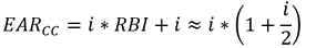
A useful concept to evaluate the consequences of different compounding frequencies is the effective annual interest rate (EAR):
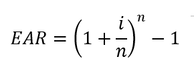
Where i is interest rate, n is the number of compounding periods per year. To see how beneficial the effects of compounding really are, we can calculate the annual “bonus interest” (BI) earned through compounding, in excess of the interest rate:
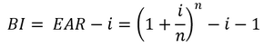
This relationship highlights the benefit of high compounding frequency, it improves the effective annual interest rate:
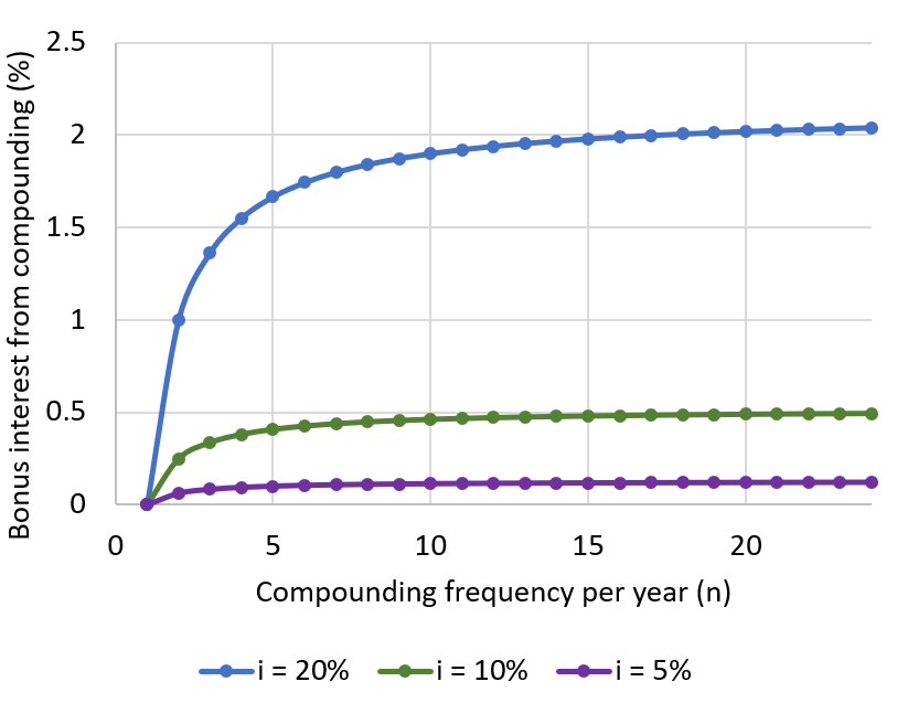
Higher compounding frequency gives additional annual bonus interest, though the value plateaus at high compounding frequency. The maximum bonus interest is achieved under continuous compounding:
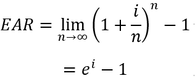
This is the maximum effective annual interest rate possible. In this case, the accumulation function (A) becomes:
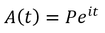
Where P is the initial principle invested. The simplified form of the continuous compounding EAR provides an opportunity to further analyze it. I define the relative bonus interest (RBI) the ratio of the bonus interest (BI) to the interest rate (i) under continuous compounding:
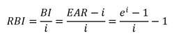
When interest rates are not extremely high, e.g. < 20%, this equation is well approximated by a simpler form:
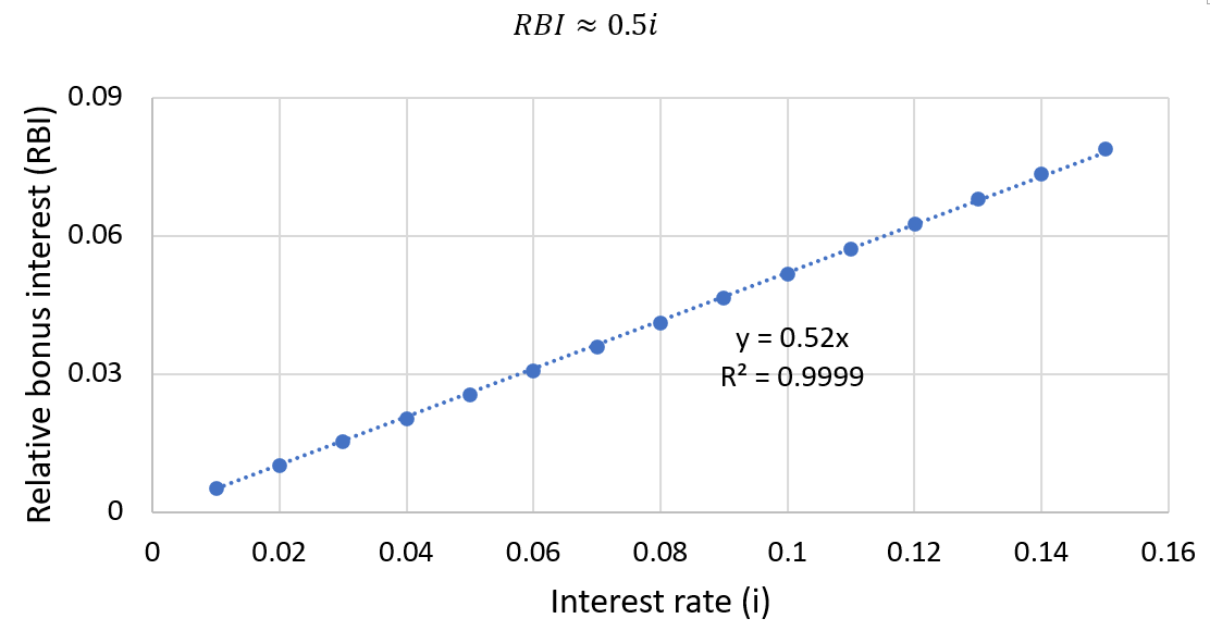
This heuristic makes it easy to determine the effect of continuous compounding without a calculator. It is convenient that this approximation only fails at high, unrealistic interest rates.
Thus, to estimate EAR under continuous compounding:
Thus, to estimate EAR under continuous compounding:
For instance, suppose continuous compounding of an annual 10% interest. Using the above approximation, we estimate an RBI of 5%, giving 10.5% EAR. In comparison, the exact value is 10.52%. Though the size of this benefit appears modest, it becomes impactful over longer timescales. For instance, at 10% EAR, $100 would appreciate to $1745 after 30 years, while the 10.52% EAR earned through compounding would yield $2010.
Real vs nominal interest and the Fischer equation
The above treatment of interest rates did not consider another factor in the time value of money: inflation. This is a process whereby the purchasing power of a currency tends to decline over time. It is useful to consider the true buying power over time, and therefore we can make a distinction between the nominal interest (i) and the “real interest” (r) after the decline in value due to inflation (π). These rates are related by the Fischer equation:
Where i is nominal interest, r is real interest, and π in inflation. When inflation is small, this real interest rate can be approximated by a simpler equation:
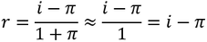
To visualize this, I plot below the real interest as a function of nominal interest at several inflation rates. The solid lines show the exact values and the markers give the approximated values.
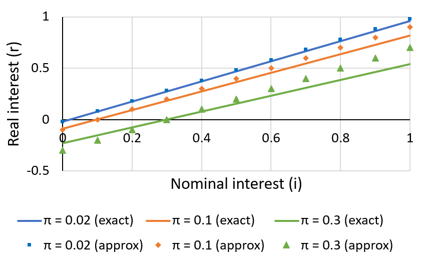
When the inflation rate is greater than nominal interest, the real interest becomes negative. When the inflation rate is small, the approximation gives good agreement with the exact equation (see π = 0.02).
The distinction between nominal and real interest has little effect on the earlier treatment of compound interest, except that the “real” interest rate is lower than the nominal one. The earlier equations could use either rate to consider the inflation-adjusted or nominal value of the investment, respectively.
The distinction between nominal and real interest has little effect on the earlier treatment of compound interest, except that the “real” interest rate is lower than the nominal one. The earlier equations could use either rate to consider the inflation-adjusted or nominal value of the investment, respectively.
Rule of 72
When thinking about the growth of an investment, a useful concept is the time required for it to double, the doubling time (td). A convenient heuristic for estimating this is called the rule of 72 (also sometimes 70 or 69.3), where 72 is divided by the percentage interest rate:

For instance, at 10% annual interest rate an investment would take around 7.2 years to double in value. The curious aspect of this formula is where the 72 comes from. I will clarify this by deriving this approximation. To begin, the doubling time is reached when the future value is twice the present value (assuming annual compounding):
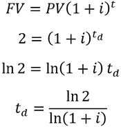
If the interest rate is small, ln (1+i) can be approximated by i, giving a simplified expression:
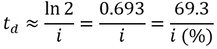
Therefore, dividing 69.3 by the interest rate as a percentage estimates the number of time units required to double the investment. Despite this result, using 72 in this model is often preferred over 69.3. There are several reasons for this. First of all, the number is easy to remember and has many useful multiples (e.g. 2, 3, 4, 6, 8, 9, and 12) which simplifies mental math. Most importantly though, increasing the value slightly from 69.3 reduces the approximation’s error around much of the commonly encountered interest rate range. To visualize this, I plot the doubling time of annual compounding as a function of interest rate and compare it with the predicted values by a 69.3 or 72 rule:
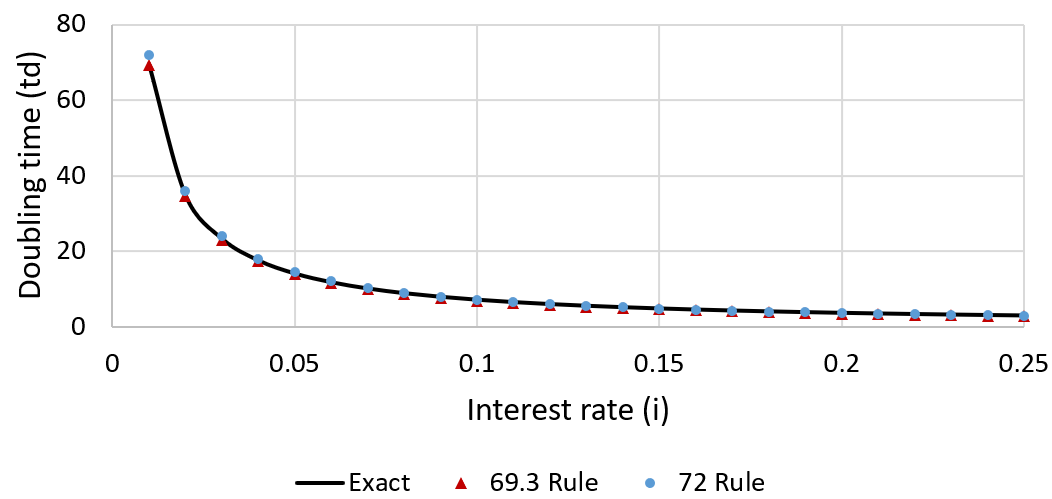
Both the 69.3 and 72 rules generally give similar times to the true values. Though subtle, the 69.3 rule performs best at very low interest rates (<0.05), increasingly underestimating the doubling time at higher interest rates. The 72 rule over-estimates the doubling time at low interest rates (<0.05) but performs better at high interest rates. To see the size of the errors more clearly, I plot the relative error against interest rate for both models:
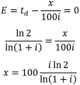
It is much easier to see in this graph that both the 69.3 and 72 rules underestimate the doubling time at high interest rates. The 72 rule performs very well between 5 and 10% interest, while at lower interest rates (e.g. <3%) a 69.3 (or 70) rule gives less error. Generally, choosing a larger constant (x) for this heuristic increases the interest rate at which it performs well. To find the optimum model parameter around a particular interest rate (i) we seek an error (E) of zero:
Plotting the optimum model parameter against interest rate:
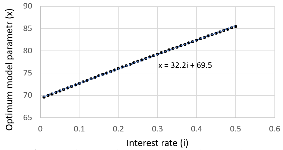
We find that the optimum model parameter increases nearly linearly with interest rate. Again, it is clear that 72 is a good choice when working between ~ 5% to 10% interest, though at very low interest 70 would be preferable. Alternatively, when dealing with unusually high interest a higher x value could be chosen. For instance, at interest rates between 20-30%, 78 would give good results.
Though the above treatment focused on annually compounded interest, continuous compounding presents an interesting special case. The result of the calculation is simpler, the 69.3 form of the equation comes out as the exact result:
Though the above treatment focused on annually compounded interest, continuous compounding presents an interesting special case. The result of the calculation is simpler, the 69.3 form of the equation comes out as the exact result:
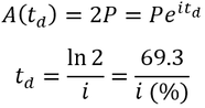
Thus, for continuous compounding at any interest rate using the 69.3 rule provides accurate doubling times.
Periodic contributions under compound interest
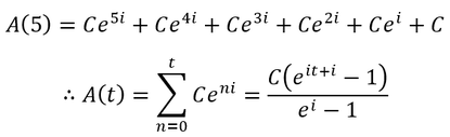
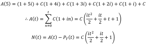
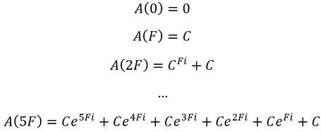
The mathematical treatment of compound interest is simplified when we consider the growth of just a single investment. However, a more complicated, realistic scenario is investing periodically in portions over time. Suppose we contribute C principle every year (t), under continuous compounding at annual interest rate i. As an example, the accumulation function after 5 years is equal to:
The amount invested at any given time is given by the total principle, PT:
Another useful quantity is the net appreciation, N, the increase in value above the total principle:
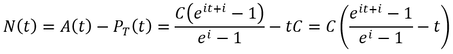
To appraise the benefit of compounding in this periodic contribution scenario, we can compare it the results without compounding, simple interest:
To visualize the consequences of these equations, I plot these accumulation functions assuming a contribution of $1000 per year and 5% interest, both for simple interest and continuous compounding:
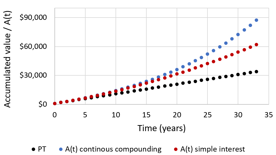
As before, continuous compounding gives a superior rate of growth compared with simple interest. Under periodic contributions the total principle grows linearly with time, simple interest gives quadratic growth, and continuous compounding achieves exponential growth.
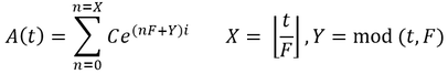
Now I extend the model, allowing contributions to be made at a frequency of every F months instead of yearly. We can utilize the above equations, grouping the time into increments of F months and expressing interest rate (i) as a monthly rate:
Now I extend the model, allowing contributions to be made at a frequency of every F months instead of yearly. We can utilize the above equations, grouping the time into increments of F months and expressing interest rate (i) as a monthly rate:
However, between time increments of F months, the next contribution has not been made yet but existing contributions benefit from additional accumulation time. For instance, consider the month after 5F months:

Thus, each accumulation term grows based on the number of months since the last contribution (Y). In addition, the number of exponential terms is given by the total number of contributions made (X), a function of the contribution frequency F. We can write the accumulation function as:
Exploring the consequences of different contribution schedules, consider three ways we could invest $12,000 dollars each year: $1000 per month, $12,000 at the start each year as a lump sum or a single contribution of $12,000 at the end of the year. I compare these three scenarios at 20% annual interest with continuous compounding:
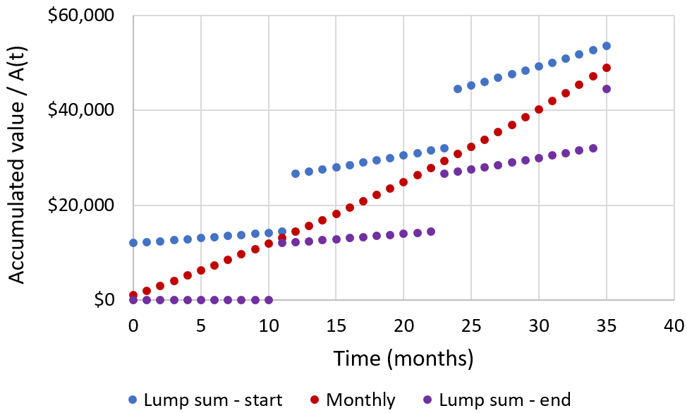
Fastest growth is achieved when the yearly $12,000 is invested at once at the beginning of the year, while worst performance is achieved when the money is invested at the end of the year. The result is easy to understand: if more of the money is invested earlier there is more time for the interest to compound. In practice, this means that regular contributions is preferable over saving the money up and investing as a large lump sum (as long as the transaction fees are low compared to the contribution size).
 RSS Feed